library(tidyverse)散布図・相関係数・単回帰分析
連続変数の二変量統計ついて学びます。
パッケージの読み込み
データの準備
学習時間(時間/日)とテスト得点(点)の調査データ(n = 80)を想定する。
set.seed(123)
n <- 80

df <- tibble(
  study_hours = runif(n, min = 0, max = 8),
  noise       = rnorm(n, mean = 0, sd = 8)
) |>
  mutate(
    test_score = 40 + 5 * study_hours + noise,
    test_score = pmin(test_score, 100)   # 上限 100 点
  ) |>
  select(-noise)

summary(df)
study_hours test_score
Min. :0.004998 Min. :32.84
1st Qu.:2.088011 1st Qu.:48.20
Median :3.765116 Median :59.79
Mean :4.011478 Mean :60.06
3rd Qu.:6.043770 3rd Qu.:68.41
Max. :7.954158 Max. :92.67 散布図
基本の散布図
2 変数の関係を探索するには,統計量を計算する前に必ず散布図を描きましょう。
ggplot(df, aes(x = study_hours, y = test_score)) +
  geom_point(color = "#534AB7", alpha = 0.7) +
  labs(x = "学習時間(時間/日)", y = "テスト得点(点)") +
  theme_minimal(base_family = "YuGo-Medium")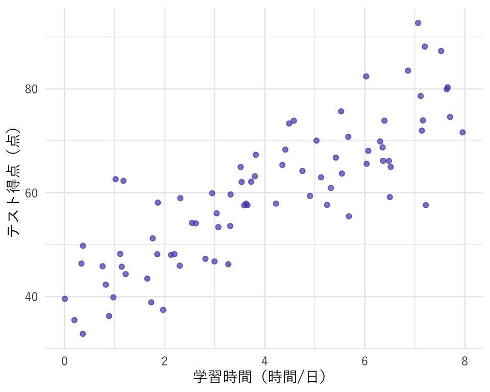
回帰直線と信頼帯(confidence band)の追加
ggplot(df, aes(x = study_hours, y = test_score)) +
  geom_point(color = "#534AB7", alpha = 0.6) +
  geom_smooth(method = "lm", se = TRUE,
              color = "#D85A30", fill = "#F0997B", alpha = 0.2) +
  labs(x = "学習時間(時間/日)", y = "テスト得点(点)") +
  theme_minimal(base_family = "YuGo-Medium")
`geom_smooth()` using formula = 'y ~ x'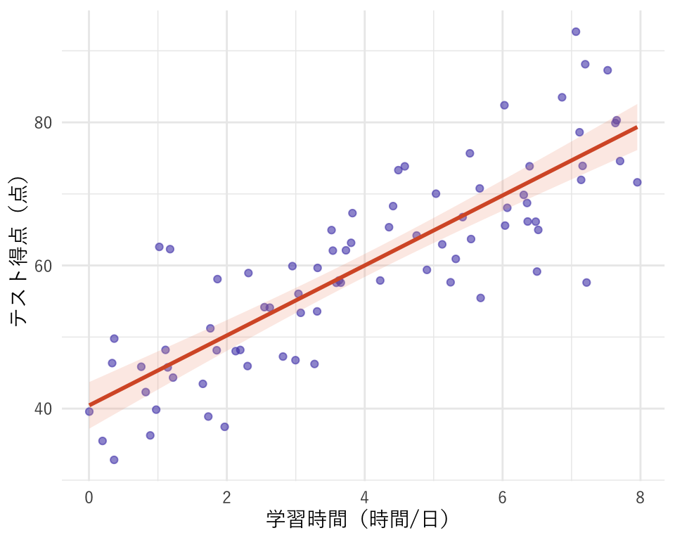
Anscombe’s Quartet:散布図を見ることの重要性
4 つのデータセットはピアソン相関係数・回帰係数がほぼ同一だが,散布図の形は全く異なる。
anscombe_long <- anscombe |>
  pivot_longer(everything(),
               names_to  = c(".value", "set"),
               names_pattern = "(.)(.)"
  )

ggplot(anscombe_long, aes(x = x, y = y)) +
  geom_point(color = "#534AB7", size = 2.5, alpha = 0.8) +
  geom_smooth(method = "lm", se = FALSE, color = "#D85A30", linewidth = 0.8) +
  facet_wrap(~ paste("Dataset", set), nrow = 2) +
  labs(x = "x", y = "y",
       caption = "各データセット:r ≈ 0.82,傾き ≈ 0.50,切片 ≈ 3.00") +
  theme_minimal(base_family = "YuGo-Medium")
`geom_smooth()` using formula = 'y ~ x'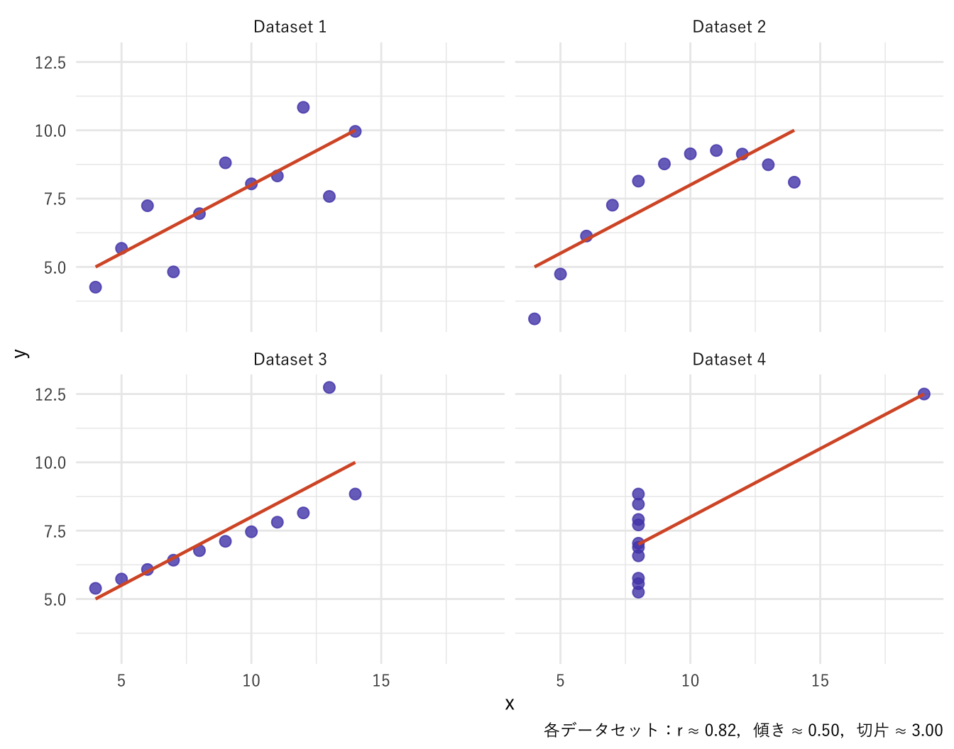
相関係数だけで判断せず,散布図で分布の形を必ず確認すること。
ピアソンの積率相関係数
定義
2 つの連続変数 \(x\),\(y\) の線形関係の強さを −1〜+1 で表す。
\[ r = \frac{\sum_{i=1}^{n}(x_i - \bar{x})(y_i - \bar{y})} {\sqrt{\sum(x_i-\bar{x})^2 \cdot \sum(y_i-\bar{y})^2}} \]
ピアソン相関係数は連続変数かつ線形関係を仮定している。
cor() による計算
r <- cor(df$study_hours, df$test_score, method = "pearson")
r
[1] 0.8418069cor.test() による有意性検定
- H₀:母相関係数 = 0(線形関係がない)
- H₁:母相関係数 ≠ 0(α = 0.05)
result_cor <- cor.test(df$study_hours, df$test_score, method = "pearson")
result_cor
    Pearson's product-moment correlation

data:  df$study_hours and df$test_score
t = 13.773, df = 78, p-value < 2.2e-16
alternative hypothesis: true correlation is not equal to 0
95 percent confidence interval:
 0.7632625 0.8958315
sample estimates:
      cor
0.8418069
p値が十分に小さく、有意に相関があるといえる。
注意:相関係数は線形関係の強さを測る指標であり,因果関係を示すものではない。
単回帰分析(OLS)
モデル
1 つの説明変数 \(x\) で目的変数 \(y\) を説明する最も基本的な回帰モデル。
\[ y_i = \beta_0 + \beta_1 x_i + \varepsilon_i, \quad \varepsilon_i \sim N(0, \sigma^2) \]
OLS(最小二乗法)は残差二乗和 \(\sum \varepsilon_i^2\) を最小にする \(\hat{\beta}_0\),\(\hat{\beta}_1\) を求める。
\[ F = \sum\left(y_i - \beta_0 - \beta_1x_i\right)^2 \]
とおいて、
\[ \frac{\partial F}{\partial \beta_0}=0,\quad \frac{\partial F}{\partial \beta_1}=0 \]
を解けばよい。 結果は次のようになる。
\[ \hat{\beta}_1 = \frac{\sum(x_i - \bar{x})(y_i - \bar{y})}{\sum(x_i - \bar{x})^2}, \quad \hat{\beta}_0 = \bar{y} - \hat{\beta}_1 \bar{x} \]
lm() によるモデル推定
model <- lm(test_score ~ study_hours, data = df)
summary(model)
Call:
lm(formula = test_score ~ study_hours, data = df)

Residuals:
     Min       1Q   Median       3Q      Max
-18.1335  -5.0409  -0.5601   4.1656  17.6749

Coefficients:
            Estimate Std. Error t value Pr(>|t|)
(Intercept)  40.4354     1.6380   24.68   <2e-16 ***
study_hours   4.8926     0.3552   13.77   <2e-16 ***
---
Signif. codes:  0 '***' 0.001 '**' 0.01 '*' 0.05 '.' 0.1 ' ' 1

Residual standard error: 7.226 on 78 degrees of freedom
Multiple R-squared:  0.7086,    Adjusted R-squared:  0.7049
F-statistic: 189.7 on 1 and 78 DF,  p-value: < 2.2e-16
出力の読み方
| 項目 | Estimate | Std. Error | t value | Pr(>|t|) |
|---|---|---|---|---|
| 切片 β̂₀ | 40.4354 | 1.6380 | 24.6851 | 0 |
| 傾き β̂₁(study_hours) | 4.8926 | 0.3552 | 13.7735 | 0 |
| 出力の項目 | 意味 |
|---|---|
Estimate(切片) |
\(x = 0\) のときの \(y\) の予測値 |
Estimate(傾き) |
\(x\) が 1 単位増えたときの \(y\) の変化量 |
Std. Error |
係数推定の標準誤差(不確かさの大きさ) |
t value |
Estimate ÷ Std. Error |
Pr(>|t|) |
係数 = 0 という帰無仮説への \(p\) 値 |
Multiple R-squared |
\(R^2\):\(y\) の変動のうち回帰で説明できる割合 |
F-statistic |
モデル全体の有意性検定(単回帰では \(t^2\) に等しい) |
係数の解釈
推定式:test_score = 40.44 + 4.89 × study_hours解釈:学習時間が 1 時間増えると,テスト得点は平均 4.89 点上がる。R² = 0.709:学習時間がテスト得点の変動の 70.9% を説明する。予測
predict() に interval = "confidence" を指定すると,推定値の 95% 信頼区間が得られる。
new_data <- data.frame(study_hours = c(1, 3, 5, 7))
predict(model, newdata = new_data, interval = "confidence")
fit lwr upr
1 45.32797 42.65917 47.99676
2 55.11319 53.35290 56.87347
3 64.89841 63.14466 66.65216
4 74.68363 72.02777 77.33949| 学習時間 | 予測得点 | 下限 (95%) | 上限 (95%) |
|---|---|---|---|
| 1 | 45.33 | 42.66 | 48.00 |
| 3 | 55.11 | 53.35 | 56.87 |
| 5 | 64.90 | 63.14 | 66.65 |
| 7 | 74.68 | 72.03 | 77.34 |
残差診断
OLS の前提(線形性・等分散性・正規性・独立性)を plot(model) で確認する。
par(mfrow = c(2, 2))
plot(model)
par(mfrow = c(1, 1))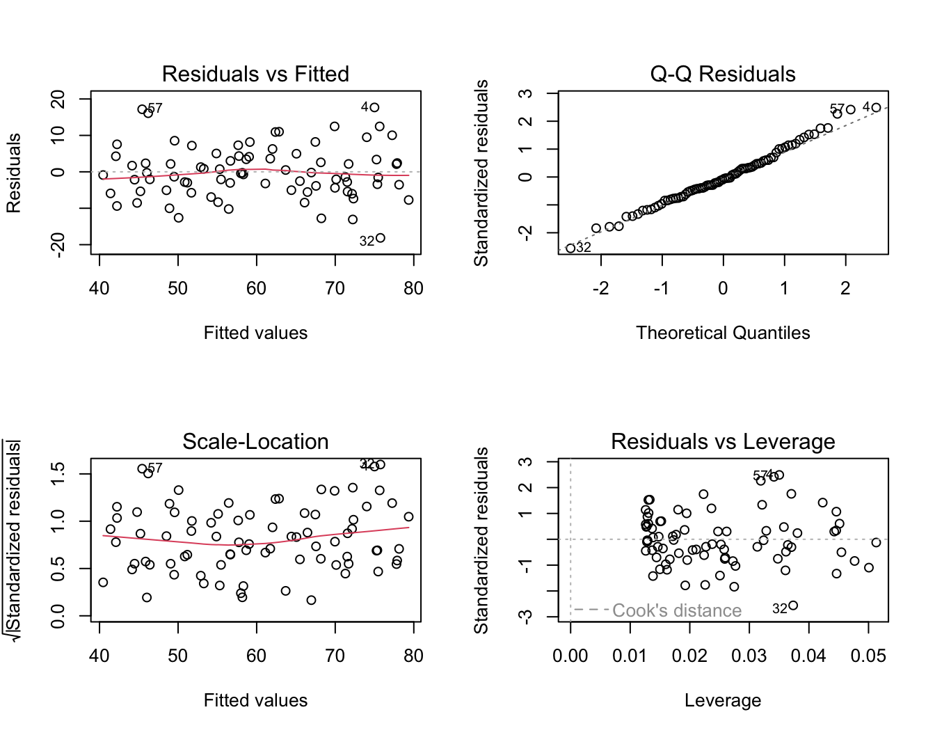
| プロット | 確認すること | 理想的な状態 |
|---|---|---|
| Residuals vs Fitted | 線形性・等分散性 | 水平な赤線,残差にパターンなし |
| Normal Q-Q | 残差の正規性 | 点が直線上に乗る |
| Scale-Location | 等分散性 | 点がランダムに散らばる |
| Residuals vs Leverage | 影響点の有無 | クック距離の破線内に収まる |
まとめ
| 関数 | 役割 |
|---|---|
| ggplot() + geom_point() | 散布図の描画 |
| geom_smooth(method = ‘lm’, se = TRUE) | 回帰直線と信頼帯の追加 |
| cor(…, method = ‘pearson’) | ピアソン積率相関係数の計算 |
| cor.test(…, method = ‘pearson’) | 相関係数の有意性検定(95% 信頼区間も出力) |
| lm(y ~ x, data) | 単回帰モデルの OLS 推定 |
| summary(model) | 係数・R²・F 統計量の出力 |
| predict(model, newdata, interval = ‘confidence’) | 予測値と信頼区間の計算 |
| plot(model) | 残差診断の 4 プロット |
次の段階へ向けて
単回帰の自然な拡張として,複数の説明変数を持つ重回帰分析がある。
\[ y_i = \beta_0 + \beta_1 x_{1i} + \beta_2 x_{2i} + \cdots + \beta_k x_{ki} + \varepsilon_i \]
重回帰では偏回帰係数の解釈・多重共線性(VIF)・モデル選択(AIC)が重要になる。